Class 1: From Excel to Stata

A first approximation: Stata as an enhanced Excel

Open Stata. Four windows organized as a consolidated workspace will automatically pop up. Nothing seems too interesting—there is only a welcome message in the Results window with some information about our version and license.

To have some action, we need to load a database. All of the windows in this workspace are instances that either:

• Can give instructions to Stata to do something (Command window), or
• Show you the output of the instructions you gave (rest of the windows).

In most cases, the things we want to do are only meaningful when there is a database loaded. So let’s load our first database to have some action!

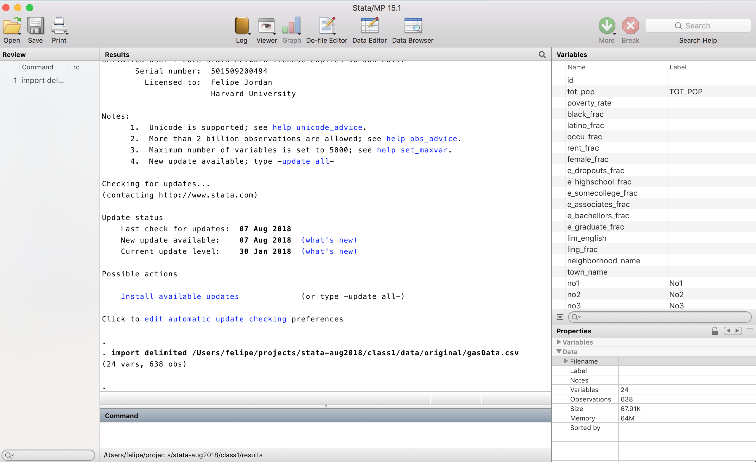
First, download and unzip the materials for this class. Select File > Import > Text Data from the top menu and browse for the file data/original/gasData.csv in the folder of this class. Click OK.

Now Stata has loaded a database. Double-click the file to inspect it in Excel (do not save afterwards!). As is generally the case in Excel, Stata follows the convention that each row represents an observation and each column a variable. In this case, observations are all the census block groups of Boston and Cambridge, and variables are some demographics from the 2010 Census and data on the status of gas leaks reported by utility companies in 2016 (more on the data later).

After loading the database, some of our windows have been populated with information:

• The Review window (left) shows the history of the commands we have given to Stata in the current session (since the last time we opened it). There is one command now, which is the result of loading the database. Whenever you give an instruction to Stata using the top menu, Stata automatically picks the relevant command and runs it in the command line.

• The Variables window (top right) lists the variables of the loaded database.
• The Properties window (bottom right) shows some information about the loaded database.
• The Results window (top center) prints the result of the instructions we have provided. In this case, it prints the import command and gives us some useful information about the result.
• The Command window is where we can give instructions to Stata using commands.

We have already indirectly introduced our first command when we imported the data (well, Stata did it for us). Now, type the following command in the Command window:

There we go! We can inspect our database. Try ordering the data by different columns (right-click on a column).

Exit the Data Editor window. Now you can see that your Review window is populated with commands! Click on one of the commands that ordered the database. The command is now written into your Command window. Try editing it to sort by another variable and type browse again to see what happens. The database should now be ordered by that variable!

We will now give Stata some commands to obtain useful information about our database. This will be our first in-class exercise.

Exercise 1: Preparing a meeting in a hurry

Assignment

Suppose you work as a policy expert in an environmental NGO that advocates for fixing gas leaks in the Greater Boston Area (such as HEET). You have received the GasData.csv database from a colleague at 11:00 AM, and you have an important meeting with members of the Boston Public Health Commission at noon. Although in this very first meeting you did not expect to have data to share, showing them some aggregate figures about the extent of the gas leak problem in Boston and Cambridge would definitely be helpful to make future cooperation with their organization more likely. By answering these questions, you will make your point clear:

1. What is the total number of leaks in each neighborhood?
2. What is the average, standard deviation, minimum, and maximum number of leaks in block groups per town, when we only consider those with at least a hundred inhabitants?
3. Is there a clear relation at the neighborhood level between the fraction of Latino population and the number of leaks per 10,000 inhabitants?

This is the email you received from your colleague:

Solution

Before starting, it is good practice to explore the database. Try the following commands:

Both describe and summarize can be followed by one or several variable names to restrict the output to those variables. If you want to know more about a command, the very first place you should ask is... Stata itself! Try:

Stata will prompt a window with very useful information. It starts with the syntax of the command, something like:

Not all commands follow this syntax, but it is pretty common. The command starts with the name of the command, followed by some arguments which may or may not be optional (they are optional if they are in square brackets). You can restrict attention to a subset of your database using the if and in qualifiers, and specify options after a comma to slightly modify the behavior of the command. Try:

Now Stata gives us more detailed information about unrepaired Grade-3 leaks (d is short for detail).

What if we are interested in seeing this summary only for Boston? Then we can use the [if] part of the command as follows:

Note the structure of what follows the if: it is a logical test. We are asking whether town_name (which is a string variable) is equal to a specific value. “Boston” is enclosed in quotes because that is how Stata knows you are referring to a specific string value, and not something else (such as another variable in your dataset).

Ok, now we will start to prepare for our meeting. We will open a log file. This file will save all the results shown in the Results window into a separate file. To do this, go to File > Log > Begin... and create a log file named exercise1 in the results folder of our class. As you might have expected at this point, Stata just printed the relevant command into the Command window and pressed Enter for us.

Now, type these commands one by one in the Command window to achieve our first goal:

Ok, we are done with the first question. Open your log file to verify that all this effort is safely saved in a file that we can print for our meeting. We are ready to start with the second part. Type these commands:

We are left with the third part. There are many ways to assess whether there is a meaningful relationship. We could calculate correlations, run regressions, build a nice table, or create a plot. Of all of them, a plot is one of the most useful, as almost everyone can understand what it represents. You can create very fancy plots using Stata (see some inspiring examples here), but for now we will explore the most basic type of plot in Stata (don't worry—we’ll get to the fancy ones in Class 4). You’ll see that even if it’s not very beautiful, the simple plot is very helpful for exploring your data.

It’s time for you to put into practice what we have learned so far! Append to your log file a series of commands that print a simple plot with the share of Latinos on the x-axis and the per-capita number of leaks on the y-axis. To guide you, I'll provide you with a list of instructions you need to translate into Stata:

1. Append your work to the log file.
2. Create a variable that stores the number of Latinos per block group, using tot_pop and latino_frac.
3. If you haven’t already done it in the previous exercise, create a variable that counts the total number of leaks per block group.
4. Preserve and collapse your database to obtain a new version where the unit of observation is the neighborhood, and you have three variables: number of Latinos, total population, and number of leaks.
5. Create two new variables: the fraction of Latinos and the number of leaks per 10,000 inhabitants.
6. Plot the relationship between both variables using plot. Type help plot to learn how to use this command.
7. Restore your database and close the log file.

Taking reproducibility seriously: Your first do file

We will create a do file now. To a first approximation, a do file is simply a file where you stack Stata commands line by line. Although simple, using do files efficiently will have a huge impact on your productivity, the quality of your empirical work, and your accountability.

We will write our first do file through a second in-class exercise.

Exercise 2: Sharing your work with your colleague

Assignment

Congratulations! The members of the Boston Public Health Commission were astonished by how well prepared you were for your meeting and are looking forward to future cooperation with your NGO! After taking a well-deserved nap, you check your inbox and see a new email from your colleague:

In the rush of preparing for the meeting, you forgot to write your commands in a do file — as you should always do — but don't panic, it's never too late. We will go step by step:

1. Open a new do file by clicking the Do File Editor button at the top of the Stata workspace.
2. Type clear all on the first line and save the do file in the scripts folder located in the folder for this class. Name the file exercise2.do. The clear all command tells Stata to remove whatever database is currently loaded into memory.
3. Write a new line in the do file that declares the working directory:

cd path_to_class1_folder

After entering this command, all file paths in the do file will be interpreted relative to the declared working directory. For example, if your working directory is /Users/Colluegue/class1 and you want to open a file located at /Users/Colluegue/class1/data/dataset.csv, you only need to type data/dataset.csv. What if the file you want is not a child of your working directory? You can either enter the full absolute path or use the double-dot notation to access a parent directory. For example, if the file is located at /Users/Colluegue/other_project/a_file.csv, you can refer to it as ../other_project/a_file.csv.

4. Write a new line in the do file to import the database as follows:

import delimited using "/data/original/gasData.csv"

In the solution, you’ll see that I used the command insheet using "/data/original/gasData.csv", c instead. That command also works, but it is deprecated. It's still important to understand it, as many Stata users continue to rely on it.

5. Write a new line that opens a log file:

log using "/data/results/exercise1.smcl", replace

Note that we use the replace option to overwrite the file if it already exists.

6. Copy and paste into the do file, line by line, each of the commands you used to answer the three questions. Skip the commands that open or close log files, but remember to end your do file with log close to properly close the log file.

Solution

You can download the solution to this exercise here (please try to solve the exercise by yourself before looking at the solution).

Congratulations! You have written your first do file. Now you can share your work with anyone who has Stata by giving them your Class 1 folder. All the other person needs to do to reproduce your analysis is change the working directory at the very beginning of the do file. This is why we prefer using relative paths to files after the working directory has been declared — it makes reproducibility easier.

Now, run the do file by clicking the icon in the upper right that says “Run.” There are four other ways to run a do file:

• You can also run only part of your code by selecting specific lines and clicking the same icon. This is extremely useful while you’re working on a do file. Note, however, that when you run only a portion of your code, you are generally not starting fresh (for example, the first line clear all is not run), and you may encounter an error if you run a line that generates a variable that has already been created.
• You can run the entire do file from the Command window using: do path_to_do_file
• You can run it from another do file using: do path_to_do_file. This is a great way to organize a large project into smaller steps and then bring everything together with a master do file that runs the full analysis. This is a good practice, as it increases the readability of your code.
• You can run it from the terminal using the Stata executable. This is an advanced technique that can be very helpful when combining multiple software tools in your workflow, or when running Stata on a server without a GUI.

From now on, all our work will be done in do files. In practice, you’ll still use the Command window to experiment and explore your data, but most of your work should be written in do files.

Before introducing the homework for this class, let me briefly highlight a few important points:

• Comment your code: Please take a look at the file exercise2-solution.do. Do you notice all those lines that start with // or *, and that block at the beginning that starts with /* and ends with */? Those are comments, and they are ignored by Stata when it reads the do file line by line. Why include lines that Stata doesn’t use? Because your code will also be read by humans — including your future self, who will thank you for leaving helpful notes. You can write one-line comments using either * or //, and multiline comments with /* to open and */ to close. It’s a good habit to start your code with a long comment that briefly explains what the code does, the required inputs, the expected outputs, the author, contact info, creation date, last update, and any other details you find useful. The more context, the better.
• Debugging your code: When you write your first version of a do file and run it, it’s very likely things won’t go as expected — and that’s totally normal. Even experienced programmers rarely get everything right on the first try. Fortunately, Stata provides error messages that help you understand what went wrong. For example, if you try to generate a variable x that already exists, Stata will display something like:

  variable x already defined

  r(100);

  This short message is usually enough to figure things out. If the message is less clear, you can click on the blue error code to get more information.

• Finding help: Especially in the beginning, you won’t always know how to solve a problem or which command to use. In those cases, Generative AIs and search engines are your best friends! Often your search will lead you to the Statalist forum, the official Stata user forum. It’s a large and active community of users, and you’ll probably find that 95% of your early questions have already been answered there. For the other 5%, you might find answers elsewhere — or you can even ask a new question on the forum. Of course, you can also reach out to the teaching team — but try to figure it out yourself first. That’s the best way to learn.

Homework: A disparity analysis

You did such a great job in your meeting that, a couple of weeks later, the Boston Public Health Commission commissioned a report from your organization. The name of the project is "A disparity analysis of exposure to gas leaks and access to gas leak repairs in the Greater Boston Area", and you have been chosen as the most capable person for the task. You’ve received the following email from your director:

To complete this homework, you will need to use three new commands:

• xtile
• save
• export

Use the help command to learn how to use these.

You can download the solution to this homework here (please try to solve the homework by yourself before looking at the solution).